The particle method discretizes fluids or solids into discrete computational units, known as particles. For solids, geometric information is represented by triangular surface elements of varying sizes. Each surface element that interacts with a particle is converted into a ghost wall particle, ensuring that both solid boundaries and fluid regions are represented uniformly in particle form. This unified representation enables numerical computations to focus exclusively on particle–particle interactions.
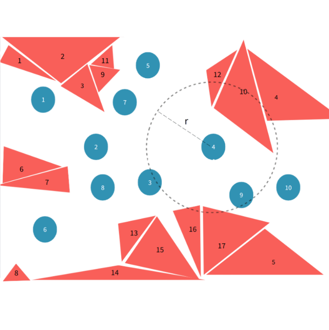
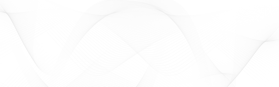
In the particle method, each particle interacts with its surroundings within a finite influence radius . A sphere of radius , centered at the particle, defines the region of influence. All particles lying within this sphere are termed neighbouring particles, and any triangular faces within this sphere are identified as neighbouring triangular faces.
Problem Description
A certain number of particles and triangular faces are randomly distributed in three-dimensional space. The interaction between particles and faces has an influence range . A sphere with radius centered at a given particle is defined, and the triangular faces within this sphere are termed the neighbouring triangular faces of that particle. The task is to identify all neighbouring triangular faces for each particle.
Implementation Approach
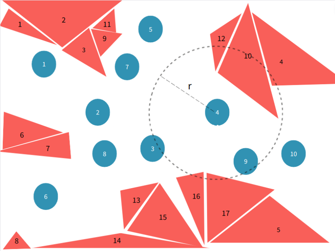
By drawing a grid in 3D space, each triangular surface in the environment is mapped onto it. One or more grid elements segment each triangular surface, transforming the positional relationship between particles and surfaces into a relationship between grid elements.
The grid cell edge length is chosen equal to the particle’s influence radius . When determining the neighbouring faces for a particle, it is sufficient to examine faces within the particle’s own grid cell and the 26 surrounding neighbouring cells in 3D. By comparing the actual distances between the particle and these triangular faces to the influence radius r, all valid neighbouring triangular faces can be efficiently identified.
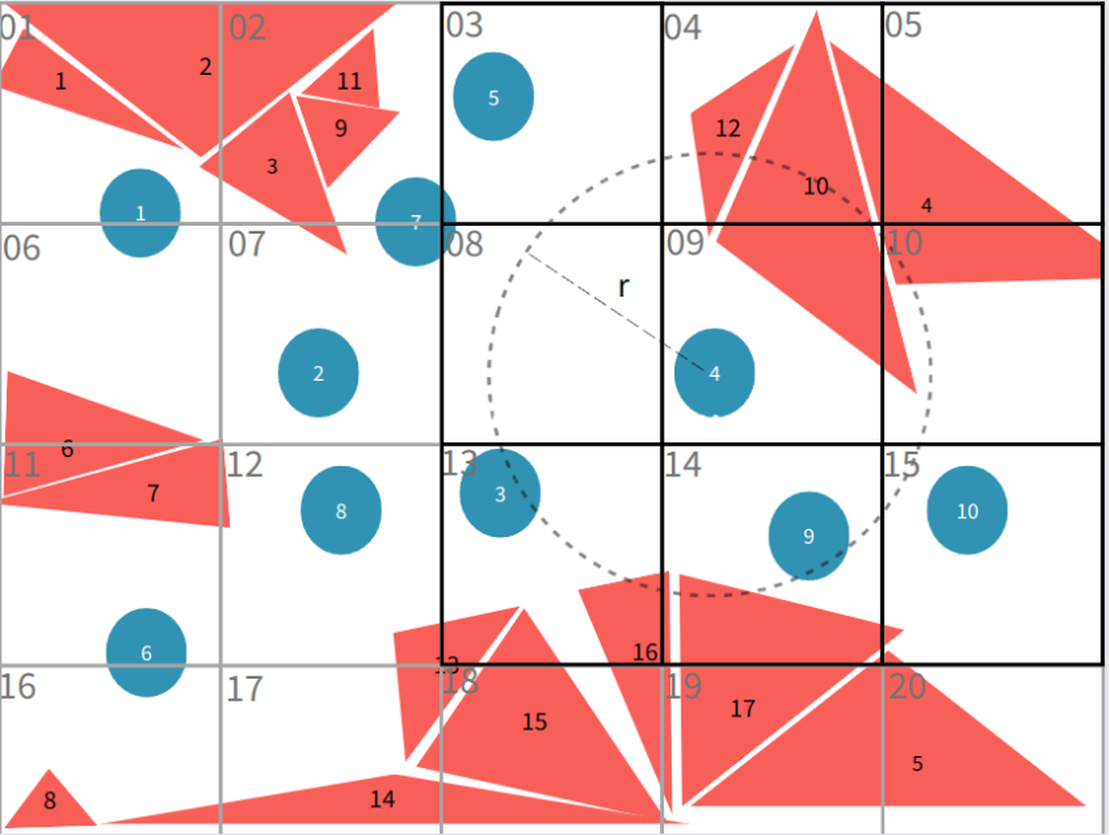
In the two-dimensional scenario, when locating the neighbouring triangular faces of particle 4, the search only needs to consider faces (4, 5, 10, 12, 13, 15, 16, 17) located in grid 9 and its adjacent grids (3, 4, 5, 8, 9, 10, 13, 14, 15). This localized search drastically reduces the computational domain and lowers time complexity.
Parallel Search
This algorithm employs a hybrid parallel approach, combining data parallelism and task parallelism. All particle data are distributed across multiple MPI processes, with each process containing full rigid body data. The grid information is traversed in parallel, calculating distances between particles and faces in neighbouring grids.
Because each operation is independent and involves no communication, it’s a prime candidate for parallel processing.
Optimisation Points
A simple mesh search for triangle IDs within neighbouring meshes may yield duplicate IDs. For instance, face ID 10 might appear in grids 4, 9, and 10 when particle 4 searches for neighbours — causing redundant computations. Hence, duplicate filtering must be implemented to ensure each triangular face is considered only once per particle.
Extensions
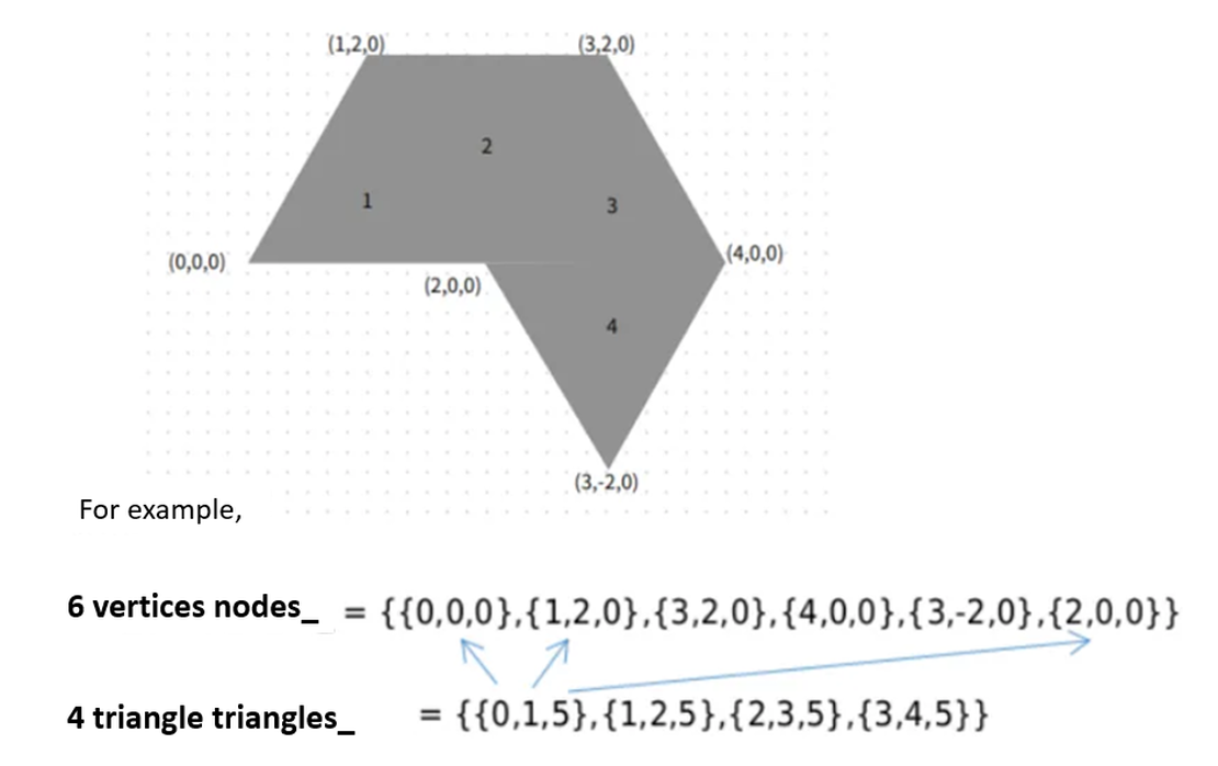
Solid Information Storage
- nodes: vertex coordinates of all triangular faces.
- triangles: vertex connectivity of each face.
Grid Information (zValue)
This algorithm employs the Hilbert curve to map three-dimensional grid coordinates into one-dimensional identifiers. The three-dimensional grid data (x, y, z) is reduced to a one-dimensional representation via the Hilbert curve. Each grid point (x, y, z) is recorded as a long integer (zValue). Morton coding converts the grid coordinates (x, y, z) into a long integer (zValue), and conversely, the grid information (x, y, z) can be retrieved from zValue via Morton coding.