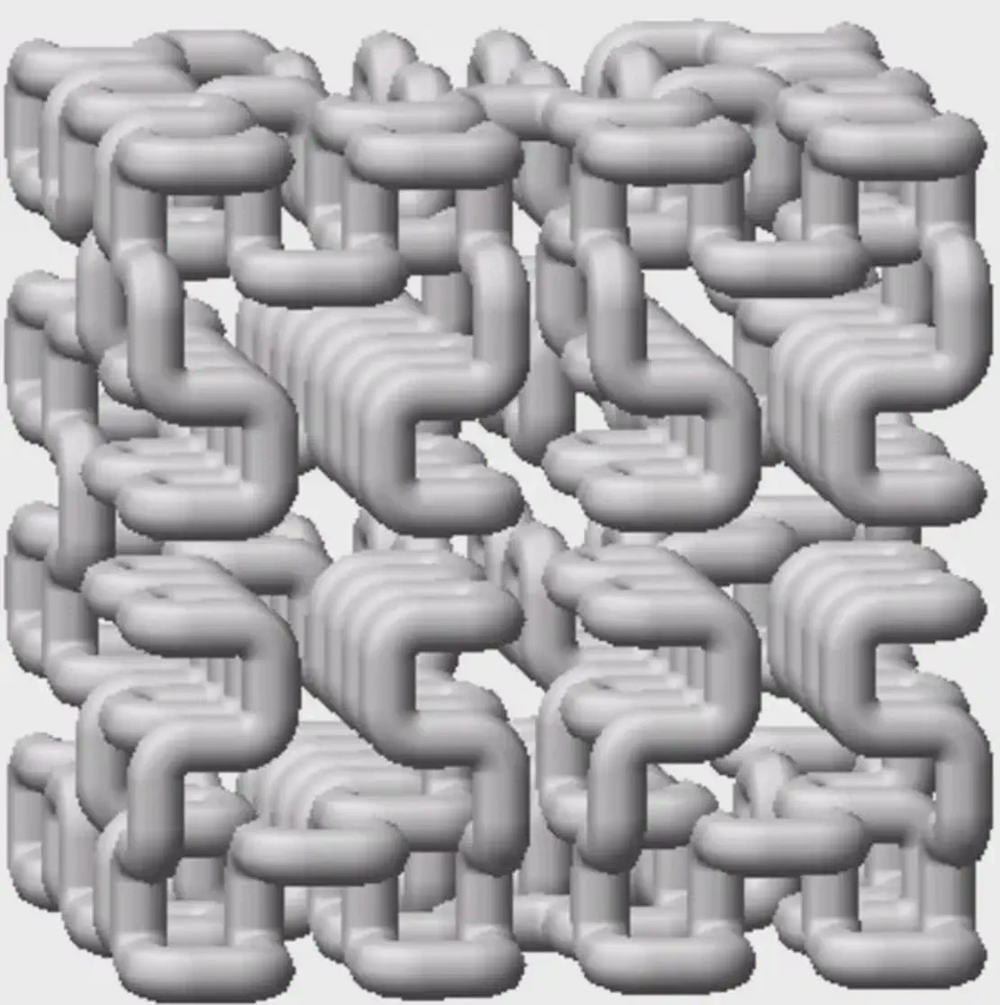
shonDy is a three-dimensional multiphysics numerical simulation software based on the mesh-free particle method. This software eliminates the constraints imposed by complex meshes during simulation by storing fluid properties on particles. Traditional mesh interactions are transformed into particle-particle interactions. These interactions have a defined influence range, termed the influence radius. A sphere centred at a particle with radius r is defined, and particles within this sphere are considered neighbours.
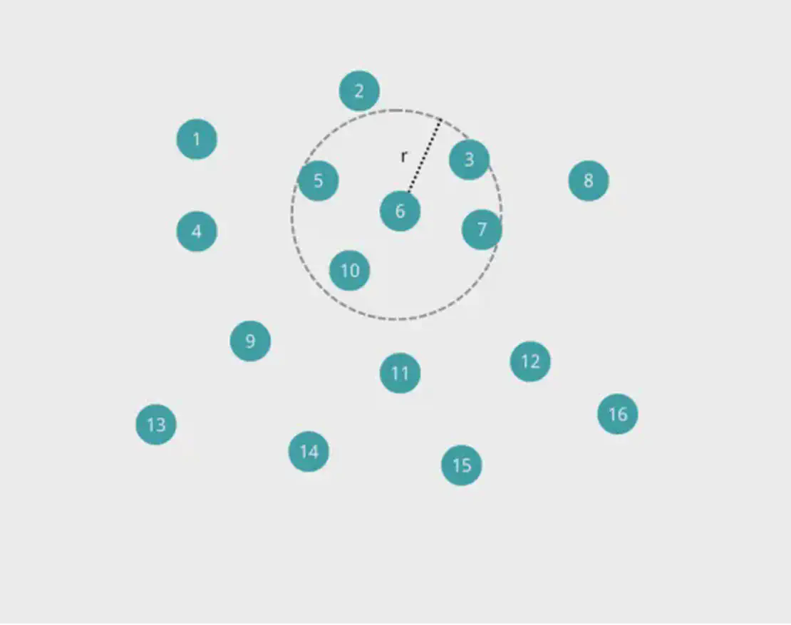
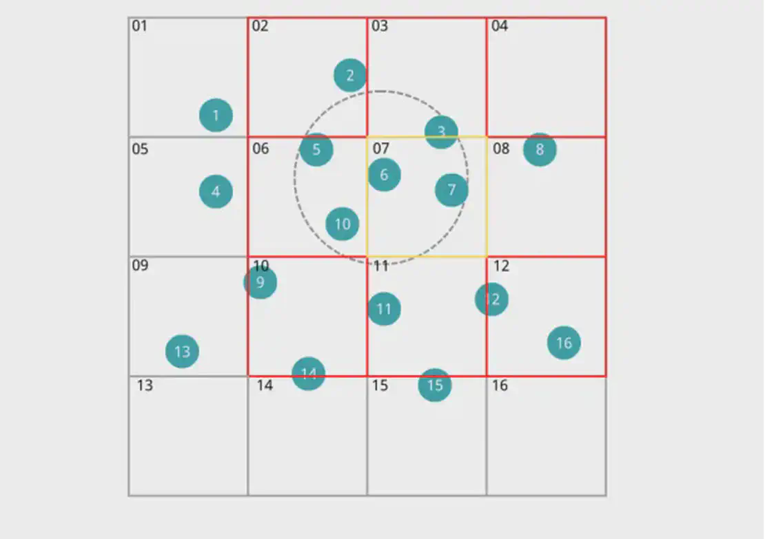
For clarity, the two-dimensional case is illustrated below:
Figure 1: Example of neighbour particles in a 2D case
Taking particle 6 as an example, its neighbouring particles have IDs 3, 5, 7, and 10.
Problem Analysis
To compute particle interactions, we must first determine each particle’s neighbours. Assuming there are n particles, a brute-force traversal approach would require a time complexity of O(n²). In large-scale projects, the number of particles can reach millions or even tens of millions, making this computation time unacceptable. Given the inherently high time complexity of this algorithm, parallel optimization based on it offers limited benefit. Therefore, a more efficient approach is required.
The crux of the problem is that each particle must traverse all other particles to find its neighbours, even though the vast majority of these traversals are unnecessary. Thus, we can reduce the time complexity by minimizing the number of particles each particle must traverse to find its neighbours. Parallelization is then based on this optimized algorithm.
Specific Implementation
We map each particle in 3D space onto a 3D grid by drawing it onto the grid. This transforms the particle-to-particle positional relationships into grid-cell-to-grid-cell relationships. The particle traversal is thus converted into grid traversal.
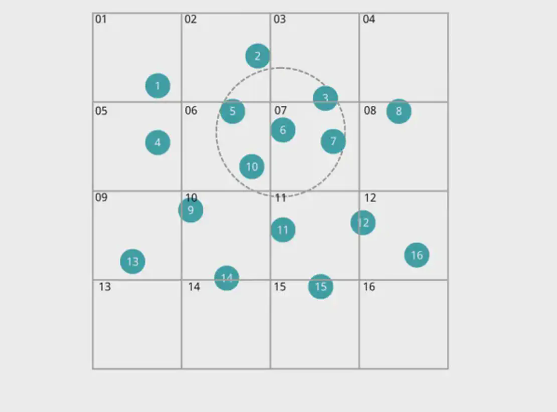
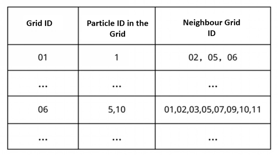
Figure 2: Mapping of particles onto grid cells
As shown in the figure, each particle ID corresponds to the grid ID it occupies.
For computational efficiency, the grid side length is typically set equal to the particle’s influence radius. When calculating a particle’s neighbours, it suffices to compute the distance between the target particle and each of the 26 surrounding grid cells, then compare each distance against the influence radius to identify all neighbouring particles.
Figure 3: Active cells for particle mapping
When searching for neighbouring particles of particle number 6, it suffices to search only among particles in the grid cells surrounding grid cell 07. This significantly reduces the search scope, thereby lowering the time complexity.
Introduction to Common Parallel Methods
1. Data Parallelism
This approach essentially involves partitioning data within a program and distributing it to different computational units for processing. The data may include both inputs and outputs. During data partitioning, the following three considerations are essential:
Load Balancing: The volume of data and computational workload processed by each computational unit should be roughly equal. Otherwise, some units may remain idle, leading to wasted computational resources.
Information Exchange: Memory configurations in parallel computing generally fall into two categories — shared memory and distributed memory. Shared memory is typically used in multi-core processors, where multiple processing units share the same memory space, necessitating measures to prevent memory conflicts. Distributed memory is commonly employed in systems composed of multiple processors, where each processor has its own memory space and requires communication during computation.
2. Task Parallelism
This approach involves dividing the problem into tasks and assigning them to different processors. Tasks must be mutually independent, with no dependencies or resolvable dependencies.
Parallelization of Neighbour Particle Search
We address this problem using a data-parallel approach. (For clarity, the following examples use two processes: process 0 and process 1)
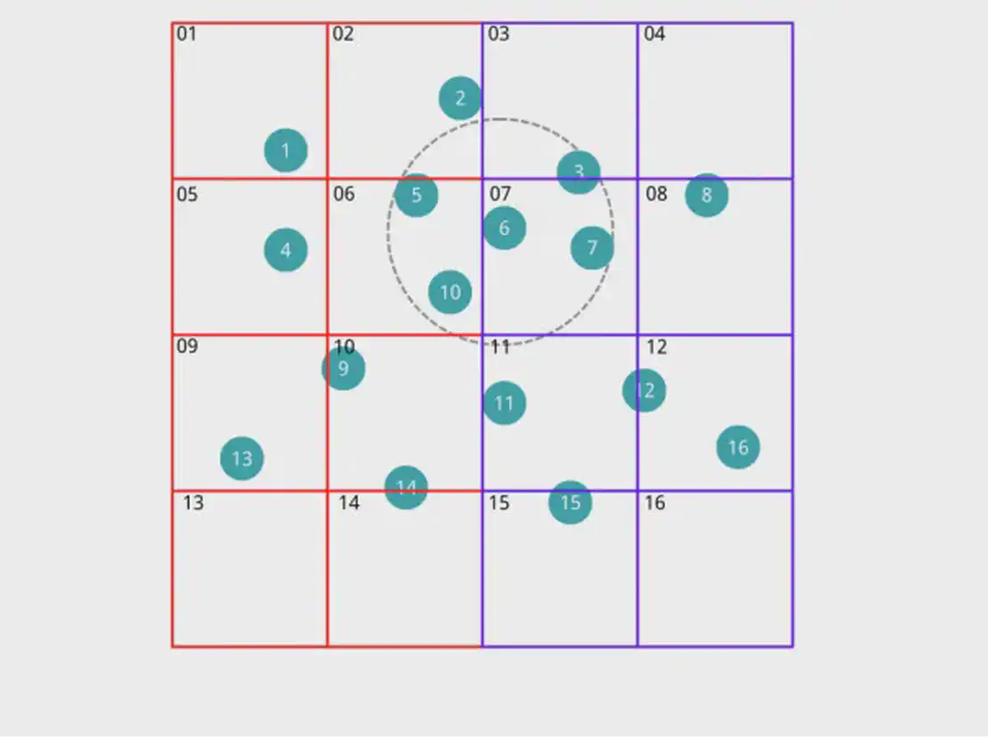
Distribute particles evenly across different processes Parallel particle distributionThe red portion on the left is assigned to process 0, and the purple portion on the right is assigned to process 1.
Calculate the grid ID for each particle and match the particle ID with the grid ID.Particle Grid IDs
Particle Information Transfer in Boundary Grids: Some grid cells lie on the boundary between two processes, such as grid 06. When locating neighbouring particles, particles in grids 03, 07, and 11 may also be neighbours of particles in grid 06. Due to the distributed-memory access model, process 0 (which hosts grid 06) lacks information about its neighbouring grids and particles, necessitating communication with process 1. The same applies to the boundary grids of process 1.
Iterate through every grid in the current process to obtain its neighbouring grids, thereby retrieving particle information from those neighbouring grids. Successively calculate the distance between particles in this grid and particles in neighbouring grids. This process involves extensive computation, with identical logical operations between particles and no information exchange, making it a prime candidate for parallel processing.
Obtain the ID of each particle’s neighbouring particles.
Extensions
GPU Acceleration Current mainstream GPUs possess substantial computational power, with performance bottlenecks primarily occurring during data read/write operations. To achieve high performance, focus on whether the program’s data structures align with GPU characteristics, typically employing contiguous storage. Additionally, minimize frequent reads/writes to global memory during program design.
Hilbert Curve Mapping This algorithm uses the Hilbert curve to map a three-dimensional grid into a one-dimensional ID.
Definition in two dimensions: The Hilbert curve is a continuous parametric curve. By selecting an appropriate function, a continuous parametric curve is drawn. When the parameter t takes values within the interval [0, 1], the curve traverses every point within the unit square, resulting in a curve that fills the entire space. The Hilbert curve is continuous yet non-differentiable.Two-dimensional Hilbert curve representation
At its core, it is a form of dimensional reduction — a curve that transforms a two-dimensional space into a one-dimensional space, extending it from two to three dimensions.
Three-dimensional Hilbert curve representation
We are ready to help!
Fill out the form
Provide your contact details and message.
We will contact you
We'll schedule a free consultation to review your goals.
Tailored Proposal
You'll receive a detailed proposal with timeline, deliverables, and pricing.
Project Kickoff
After approval, we give you direct access to our engineers.
How a Trial Request works:
Fill out the form
Select the products you want to try and fill out the form.
We will contact you
Our team will follow up with installation and activation details.
Test your product
After reviewing the product we can find a fitting license for you.