In the context of the automotive industry, wading or fording refers to a car moving through relatively deep water at a low velocity, such as crossing rivers or flooded roads. The depth a car can safely wade is crucial and is measured as the distance between the tire contact point and the engine’s air intake system. This measurement is essential to prevent water ingestion and safeguard against engine issues during such maneuvers.
Case description
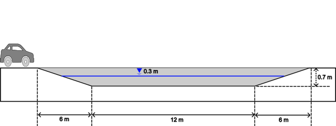
In this case, the wading scenario described above will be simulated. During the simulation, the car will travel a channel with a depth of 30 cm. The dimensions of the channel are illustrated in the figure below. Two different velocities were chosen for the simulation: 2 m/s, which corresponds to around 7 km/h, and 3.33 m/s, which corresponds to 12 km/h.
Geometry
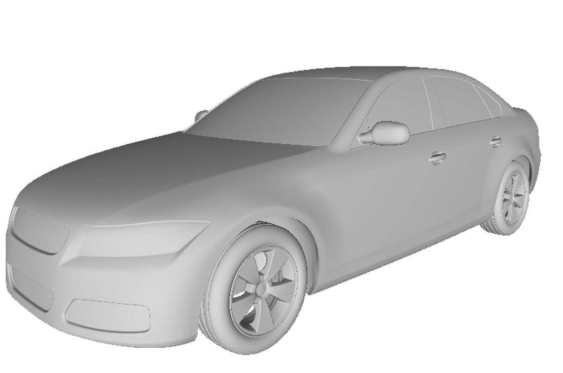
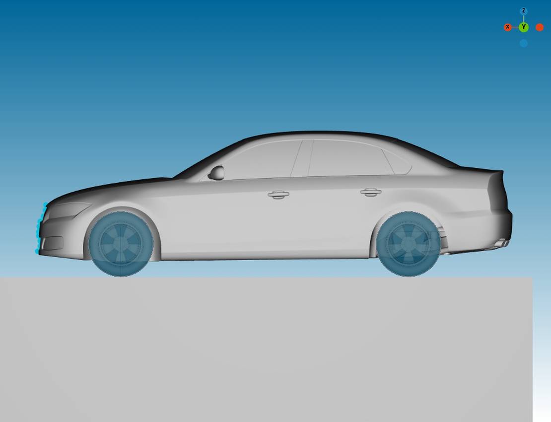
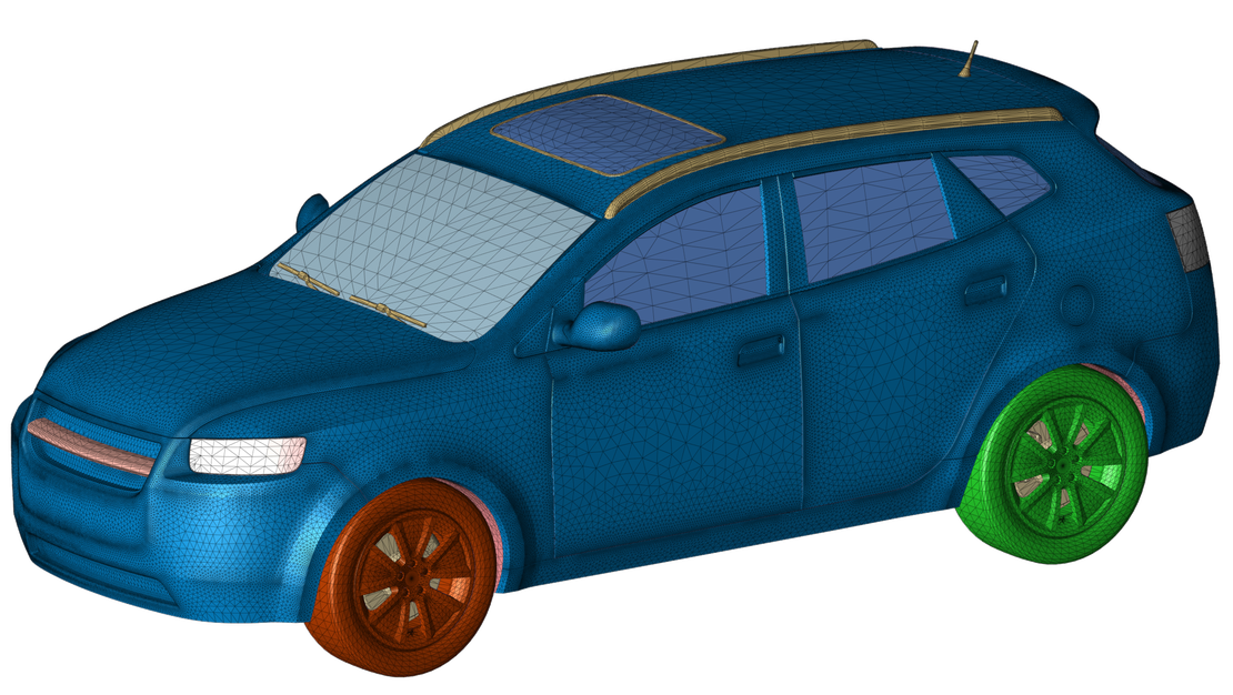
The channel’s geometry was generated based on the above sketch using shonMesh, while the car’s geometry is the so called DrivAer Model, which was developed at the Institute of Aerodynamics and Fluid Mechanics at the Technische Universität München. This model serves as a generic representation designed to bridge the gap between overly simplified models like the Ahmed body and intricate production cars. For this simulation, the DrivAer model was configured with the following specifications:
- Notchback as the top
- Detailed underbody
- Mirrors included
- Wheels present
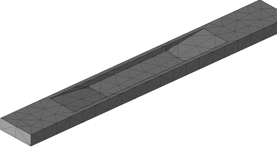
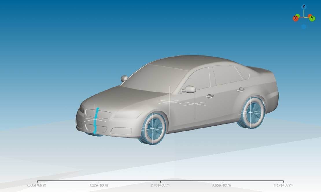
The STL file can be observed in the figure below, along with the mesh of the channel.
Case set-up
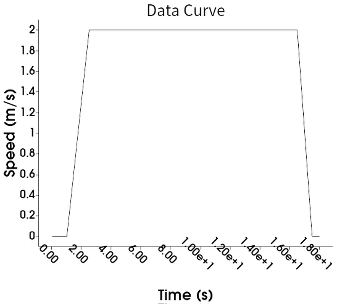
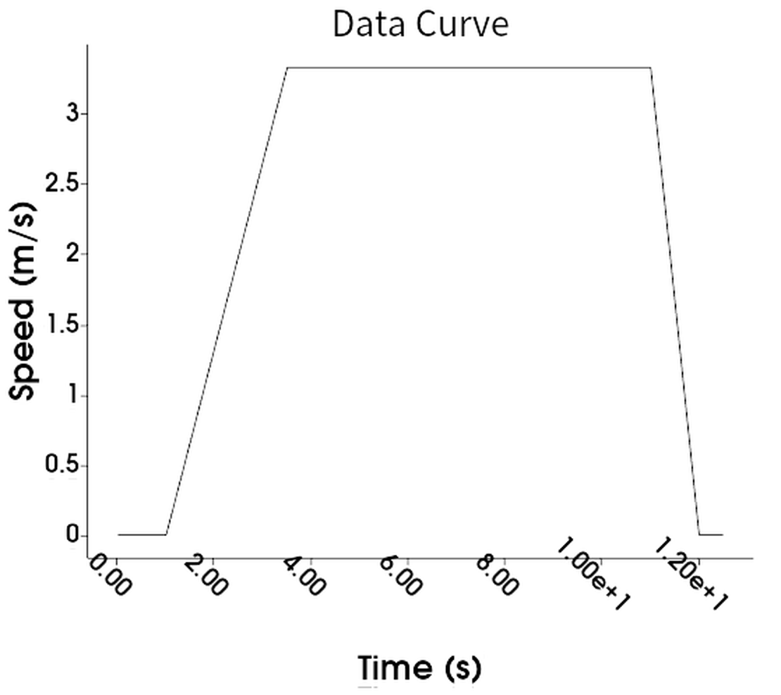
In the first simulation, the car initiates movement after 1 second, accelerates from 0 to 2 m/s in 2.5 seconds, maintains this velocity for the next 15 seconds, and comes to a stop after 18 seconds. The total calculation time is thus 18 seconds, representing the duration needed to traverse the entire channel. In the second simulation, with a higher car velocity of 3.33 m/s, the car only takes 12.5 seconds to pass through the channel, resulting in a shorter total simulation time. The precise velocity profiles can be observed in the diagrams below.
The set-up of the liquid region was the same for both simulations: A total of 15.943 m3 of liquid, equivalent to a 30 cm height, is present in the channel. For this simulation, a fluid particle radius of 1.26 cm was used, resulting in a total of 1 million particles.
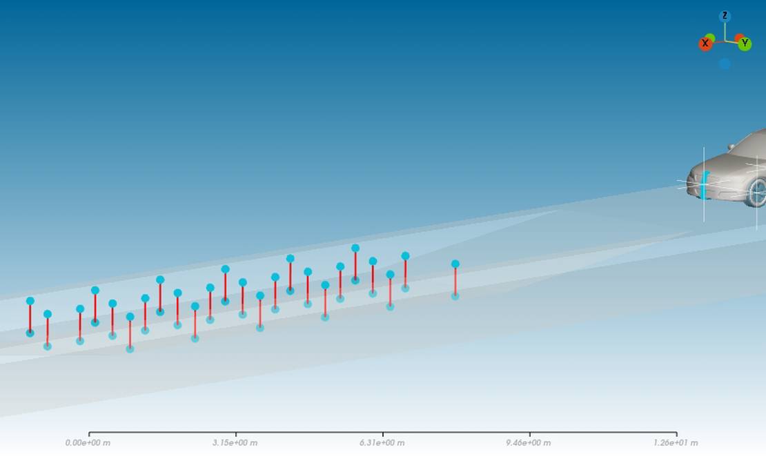
Various sampling methods were used, including:
- Sampling points at the centerline of the car
- Sampling windows around the wheels
- Sampling lines within the channel
These samplings are depicted in the figures below.
Results
General overviews of the simulations are presented in the videos below. The top row displays the slow car, while the bottom row showcases the fast car. The two top views (videos on the right) nicely illustrate the differences in the spreading of the front wave: The velocity of a surface wave in shallow water can be approximated using the formula
where g is the acceleration due to gravity, and h is the depth of the water.
In the video of the slower car, it is evident that on the ramp, where the water is less deep, the wave propagation is smaller than the car’s velocity; the wave front consistently remains at the front of the car. At the bottom of the channel, the wave is slightly faster than the car, hence it outruns the car. In the second simulation, the car is always faster than the propagation speed of the wave, hence the wave front is consistently at the front of the car.
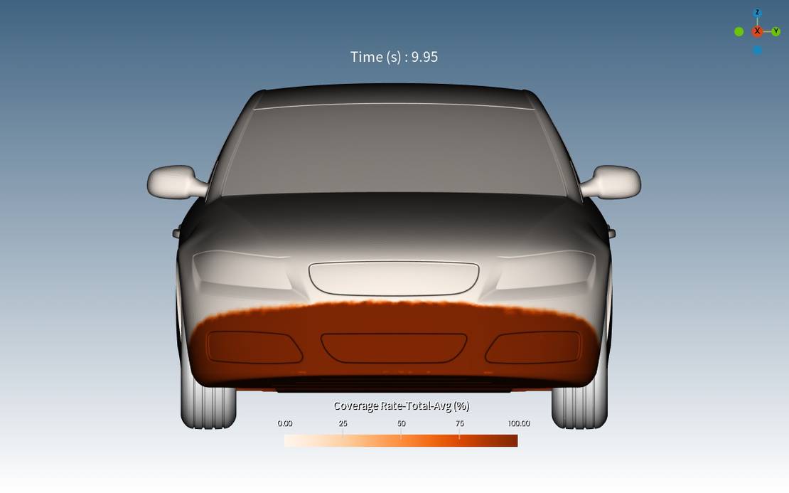
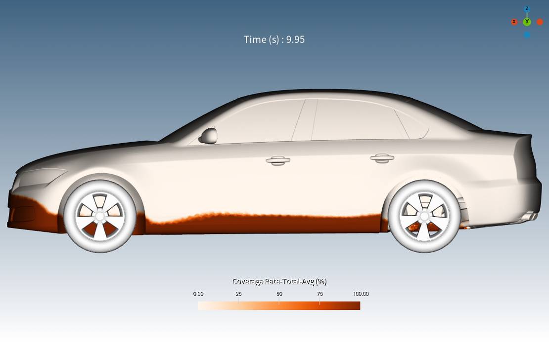
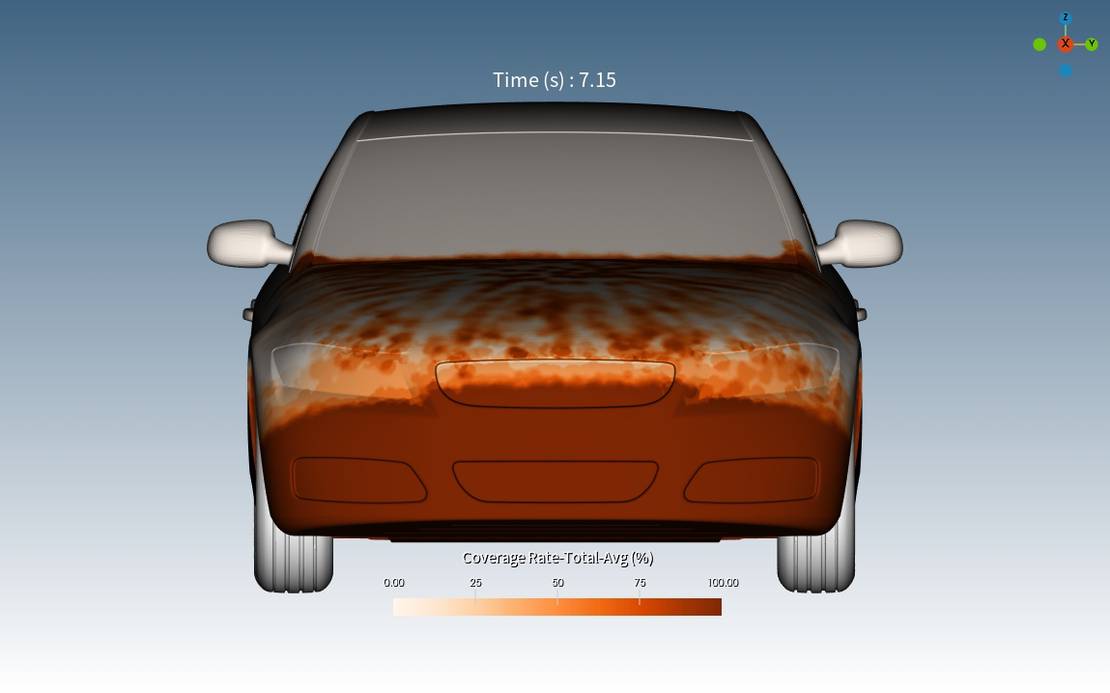
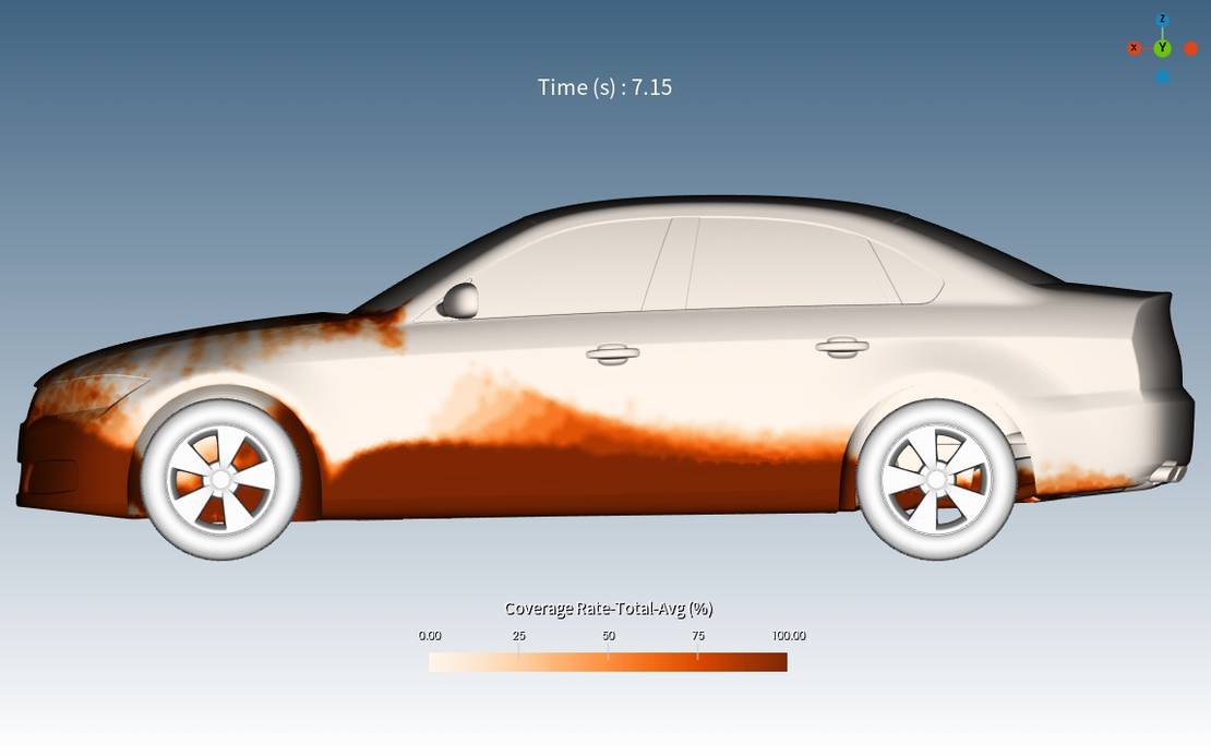
The images below display the coverage ratio on the car. Here, shonDy’s built-in time-averaging filter is used, allowing users to visualize not only the current value, in this case, the coverage ratio, but also an averaged value over a specific time. In the presented figures, the coverage ratio was averaged over 0.25 seconds to provide a clearer understanding of where the water wets the car.
Again, the top row belongs to the slower car, whereas the bottom row belongs to the faster car. Comparing the two velocities, it becomes clear that there is a difference in the distribution pattern of the coverage ratio. With a higher velocity, the car has to deal with a much higher wave, which leads to a coverage ratio over nearly the complete front of the car. This would probably lead to water in the engine compartment, which could block the air intake and causing a malfunction of the engine. On the other hand, in the case of the slower car, the water only covers the lower half of the front, meaning a much lower risk of an engine shutdown. The side view also reveals a difference: In the case of the faster car, the water level is also higher near the front doors of the car.
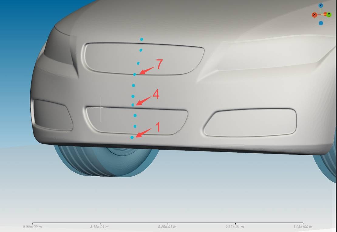
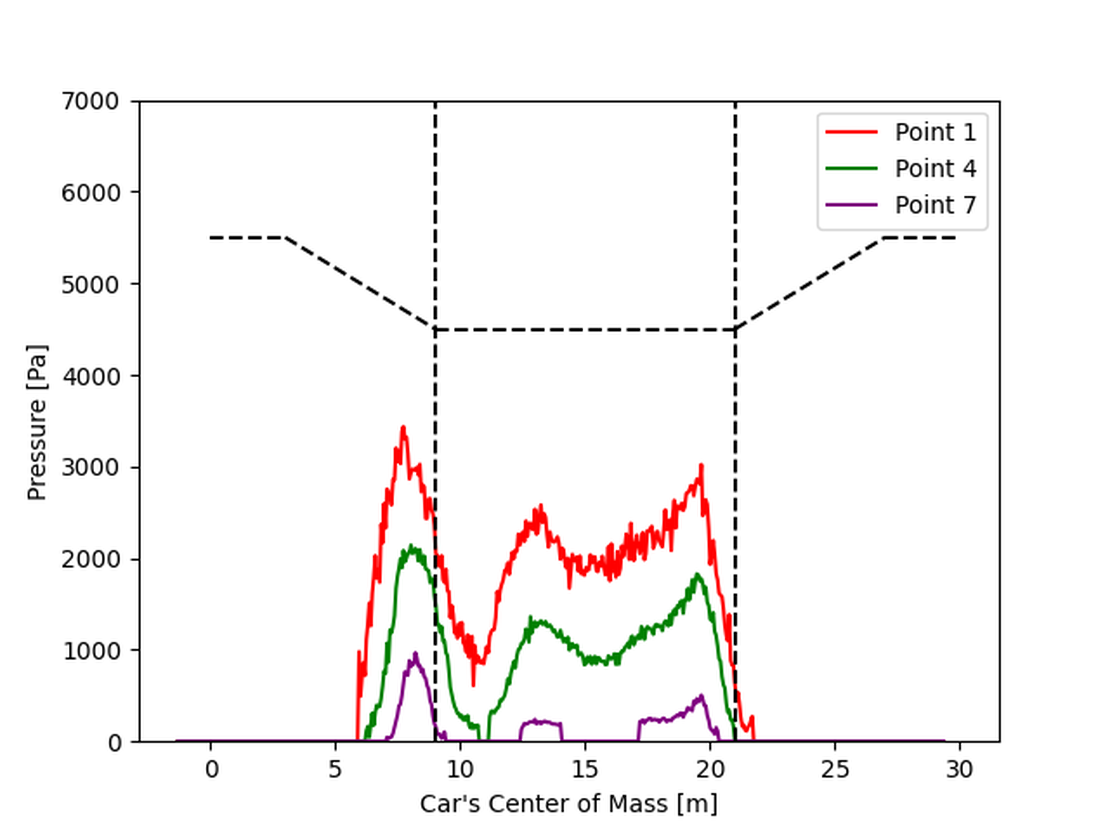
As seen in the detailed picture below, the sample points are situated at the centerline at front of the car, recording the pressure over time. To enhance comparability, the diagrams do not display pressure over time but over the position of the car’s center of mass (in x-direction). For orientation, the outline of the channel is depicted along the x-axis.
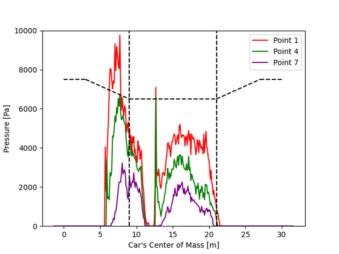
In general, it can be observed that the lowest point on the car encounters the highest pressure, while the pressure decreases at higher points. Additionally, at higher velocities, the car experiences higher pressures overall.
For higher speeds, the pressure diagram indicates that the initial impact generates the highest pressure. This impact is strong enough to push the water away from the car, creating a significant initial wave. Around 12 meters, the car catches up with this wave, and its front comes into contact with the water again.
In contrast, at lower speeds, the pressure peak is much smaller. Due to the car’s reduced velocity, the main wave created during entry moves ahead of the car, resulting in less water accumulating in front of it. Consequently, the pressure graph for the slower car shows that point 7 remains out of contact with the water for most of the time after the car is fully in the waterway.
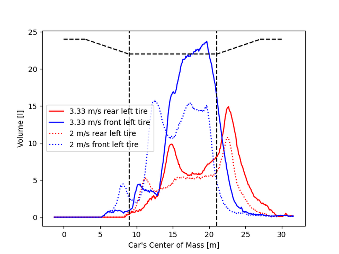
The figures below illustrate how the volume samples could be utilized. In the right picture, we observe the locations of the volume samples for the left tires. In the diagram, the fluid volume in the sample over the car’s position is depicted. Generally, the front tires have a significantly larger amount of water to contend with compared to the back tires. This aligns with the figures above where we can see the coverage ratio. From that picture, it’s evident that water accumulates at the front of the car, while in the wake of the accumulation, the rest of the car experiences a comparable low water level.
When comparing the high and low-speed simulations, we observe a similar situation as above: At higher speeds, both the front and rear tires have to deal with a higher amount of water.
Extended Scenario: 40 cm Water Depth and Convoy Simulation
The previous scenarios established a baseline at a water depth of 30 cm. To explore even more demanding wading conditions and the limits of vehicle capability, the water depth was increased to 40 cm while keeping the velocity at 3.33 m/s. This combination represents a significantly more challenging situation and reveals the point at which the compact DrivAer model reaches its wading limits.
Compact passenger car at the Limit: Buoyancy-Induced Lift
At 40 cm water depth, the volume of water displaced by the DrivAer increases substantially. As can be seen in the video below, the water already overtops the engine hood at the entry of the channel, even more than in the 30 cm case. In the video, the red color indicates the coverage ratio, reflecting the extent to which the car surface is wetted. The greater submersion depth also subjects the front of the vehicle to considerably higher buoyancy forces. Combined with the dynamic pressure generated at 3.33 m/s, these forces are sufficient to exceed the front axle load of the car. As a consequence, after approximately half the channel length, the front of the car lifts off the ground. Since the vehicle is simulated as rear-wheel drive, it retains its propulsion and completes the channel crossing in the simulation. From an engineering standpoint, however, the front axle lift-off constitutes a practical failure: the vehicle becomes uncontrollable, and a combustion engine would likely have ingested water through the air intake well before this point, causing a loss of propulsion.
This behavior illustrates a fundamental limit of compact passenger cars in deep-water wading scenarios: the relatively low front axle load and limited ground clearance make the front of the vehicle susceptible to buoyancy-induced lift once water depth exceeds a critical threshold.
SUV Model: Better Wading by Design
To provide a reference vehicle that can handle the 40 cm scenario, a generic SUV geometry was introduced. Compared to the DrivAer, the SUV features a higher ground clearance, a longer and wider body, and greater overall mass. These properties translate directly into improved wading performance. The heavier front axle load resists the buoyancy forces that caused the DrivAer to lift, while the larger body channels water gradually to the sides, reducing the net upward pressure on the vehicle. A comparison between the dimensions of the two car models can be seen in the table below:
| Parameter | SUV | DrivAer Model |
|---|---|---|
| Ground clearance | 0.3 m | 0.15 m |
| Wheelbase | 3.5 m | 2.8 m |
| Width | 2.1 m | 1.6 m |
| Weight | 2500 kg | 1500 kg |
The SUV successfully traverses the full 40 cm channel at 3.33 m/s without losing wheel contact. The coverage ratio on the front of the SUV is high, but the wave remains below the critical intake height due to the vehicle’s elevated ride height. In addition, the wave remains concentrated toward the front of the vehicle, resulting in a comparatively low coverage ratio along the sides of the SUV.
These characteristics make the SUV a suitable lead vehicle for the convoy scenario examined in the following section.
Convoy Simulation: SUV Leading, DrivAer Following
Having established that the DrivAer exceeds its practical wading limit under these conditions, the question arises whether a cooperative scenario can change this outcome. Both vehicles were simulated together in a convoy, with the SUV positioned in front and the passenger car following approximately 1.3 m behind.
As the SUV moves through the channel, it displaces a large volume of water, creating a sheltered zone of reduced wave activity and calmer surface conditions in its immediate wake. This “wave shadow” significantly reduces the hydrodynamic loading experienced by any vehicle traveling behind it.
The passenger car, sheltered within this wave shadow, encounters water conditions closer to the 30 cm baseline than to the full 40 cm depth. As a direct result, the buoyancy forces at the front axle remain below the critical threshold and the DrivAer maintains ground contact throughout the entire channel.
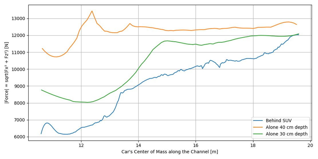
The diagram below shows the fluid force acting on the chassis plotted against the car’s center of mass position. The plotted range of 10.5 m to 19.5 m covers the horizontal section of the channel, excluding the entry and exit ramps. It is evident that the forces on the passenger car in the convoy case are even lower than in the 30 cm baseline scenario. Furthermore, the force in the convoy case rises gradually along the channel, approaching the single-vehicle level toward the exit. This indicates that water displaced by the SUV’s bow wave is directed toward the rear, incrementally increasing the hydrodynamic loading on the following passenger car.
The comparison below presents the coverage ratios for two cases side by side: the DrivAer alone at 40 cm and the convoy case at the same depth. Both images were taken at the same position along the channel, shortly before the front axle lifts off in the single-vehicle case.
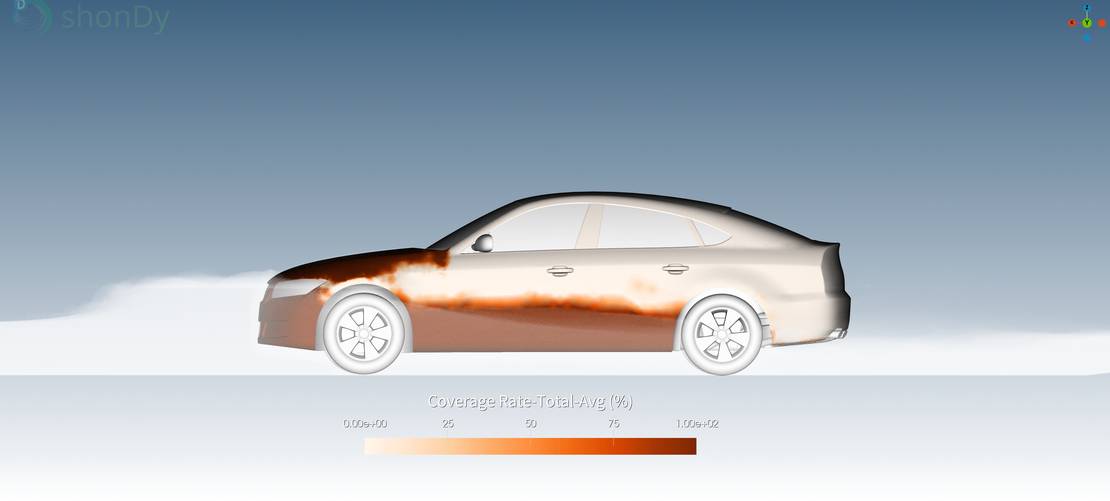
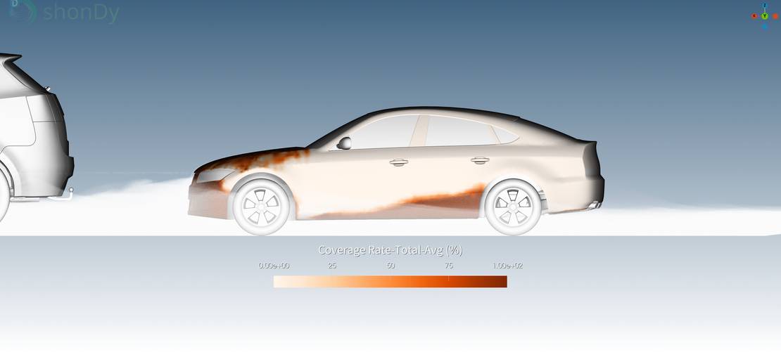
This result demonstrates that vehicle interaction during wading is a meaningful factor in assessing real-world crossing capability. The convoy arrangement effectively reduces the hydrodynamic loading on the following vehicle to levels comparable with the less severe 30 cm baseline, enabling a crossing that would not be feasible for the passenger car alone.
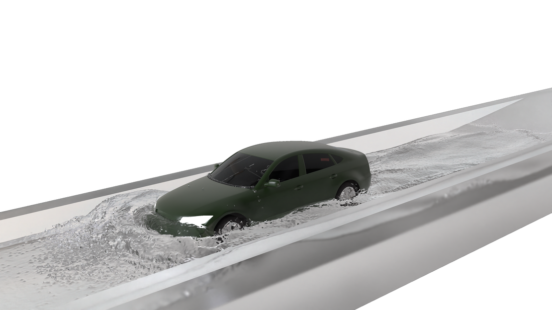
Rendered Visualization
The analyses above used shonDy’s standard visualization to keep the engineering results as clear as possible. The video below shows the same convoy simulation as a high-quality rendered output, providing a visual summary of the findings discussed above.