Improving Accuracy in the Lumped-Parameter Thermal Network (LPTN) Method

In the previous article, we introduced the fundamental principles of the Lumped-Parameter Thermal Network (LPTN) method and demonstrated how it can be used to model heat transfer using equivalent thermal resistances. The one-dimensional heat transfer example illustrated how the LPTN method can accurately predict temperature distributions in systems without internal heat sources. However, when volumetric heat generation is introduced, the LPTN method tends to overestimate the temperature.

Since the LPTN approach is widely applied to motor temperature simulation, where various motor losses are modeled as internal heat sources, enhancing its accuracy for such problems is critical. This article explores several methods to improve the LPTN model when volumetric heat sources are involved.

1. Research Case

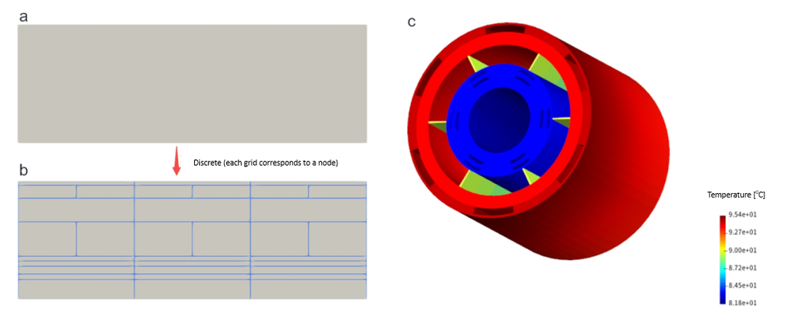
The study uses the same solid block case introduced in the first article as the research example.

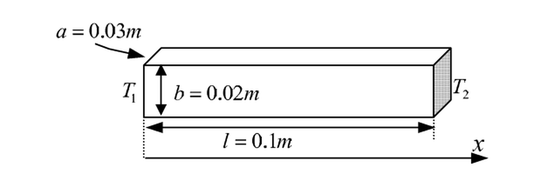
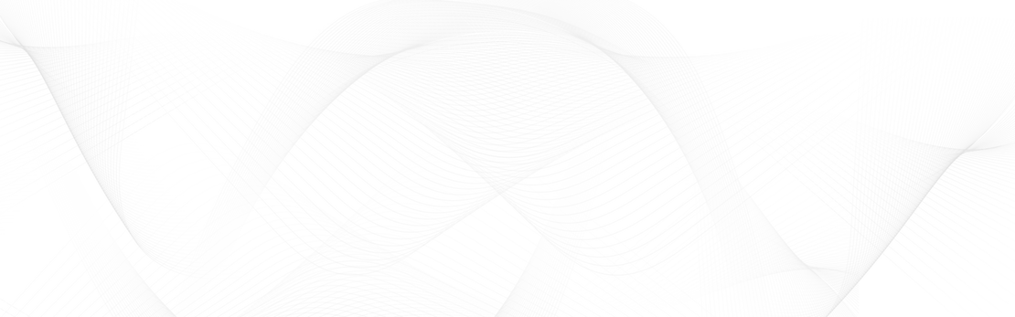
Figure 2: Thermal Network Diagram of the Solid Block

A solid rectangular block is maintained at constant temperatures $T_1$ and $T_2$ at its two ends, while being subjected to a uniform volumetric heat source. Heat transfer occurs along the x-direction of the block. The geometric configuration and the corresponding three-node thermal network representation are illustrated in Figures 1 and 2.

1.1 LPTN Method

According to the LPTN method, the temperature relationships and heat fluxes can be derived from the control equations described in Part 1.

\sum_{j=1}^{n} \dot{Q}_{ij} + S_i = \rho_i V_i C_{pi} \frac{dT_i}{dt} \tag{1}

By substituting the thermal resistances and heat generation terms, we obtain the temperature distribution within the simplified thermal network.

1.2 Analytical Solution

The analytical solution to the same problem can be obtained from the one-dimensional steady-state heat conduction equation with a volumetric heat source:

\frac{d^2 T}{dx^2} + \frac{\dot{q}}{k} = 0 \tag{2}

Boundary conditions:

T(0) = T_1, \quad T(L) = T_2 \tag{3}

Integrating twice yields:

T(x) = -\frac{\dot{q}}{2k}x^2 + C_1x + C_2 \tag{4}

The constants $C_1$ and $C_2$ are determined using the boundary conditions.

1.3 Comparison of Results

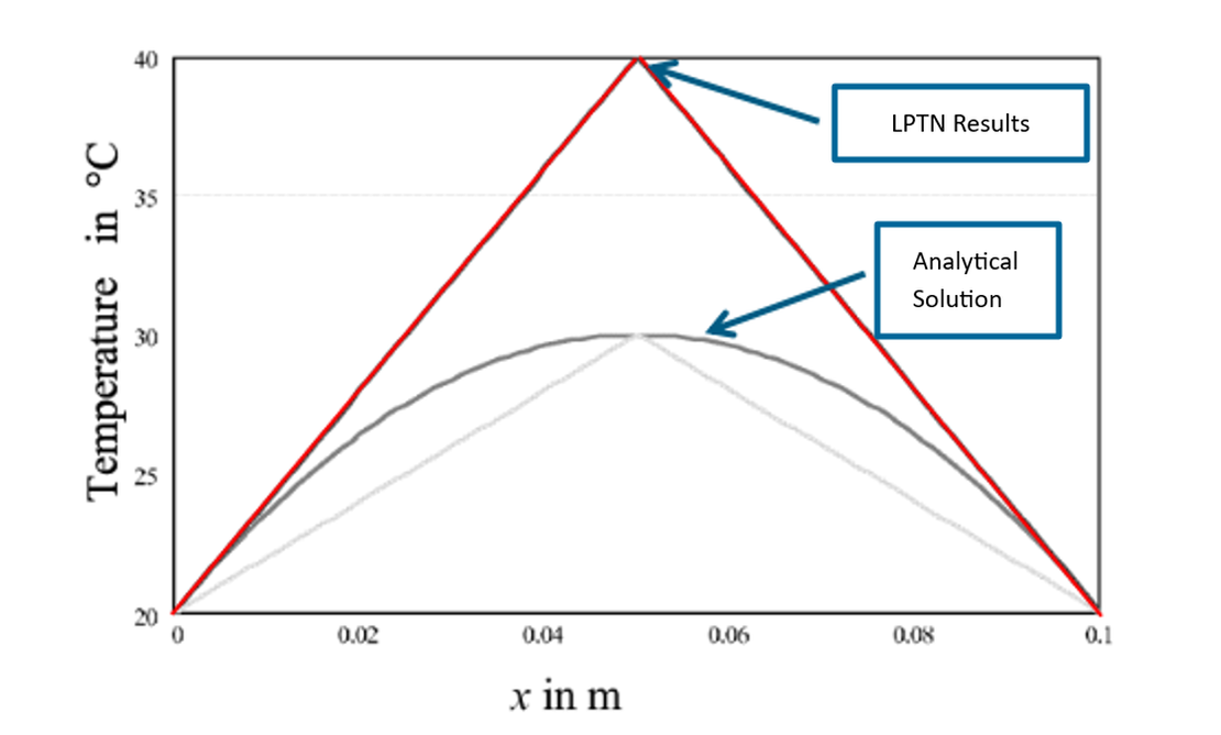
Figure 3: Comparison between LPTN and analytical results

As illustrated in Figure 3, the temperature predicted by the Lumped-Parameter Thermal Network (LPTN) method is significantly higher than that obtained from the analytical solution.

This discrepancy occurs because the volumetric heat source is distributed throughout the solid, whereas the LPTN method concentrates the entire heat source at a single network node—essentially treating it as a point source. As a result, the midpoint temperature is artificially elevated, leading to an overprediction relative to the analytical result.

2. Correction Methods

To address the overestimation of temperature in cases involving volumetric or strip heat sources, three improvement methods are proposed:

Correcting Heat Sources
Adding Additional Thermal Resistance
Increasing Node Count

2.1 Correcting Heat Sources

The primary cause of overestimation is the neglect of the spatial distribution of the volumetric heat source. If the total heat is represented more accurately within the network, the temperature prediction can be improved.

Research indicates that, although the analytical heat flux varies across the domain, its rate of change remains uniform. Therefore, adjusting the applied heat source in the LPTN model, such as reducing it to half the original magnitude, aligns the results with the analytical solution.

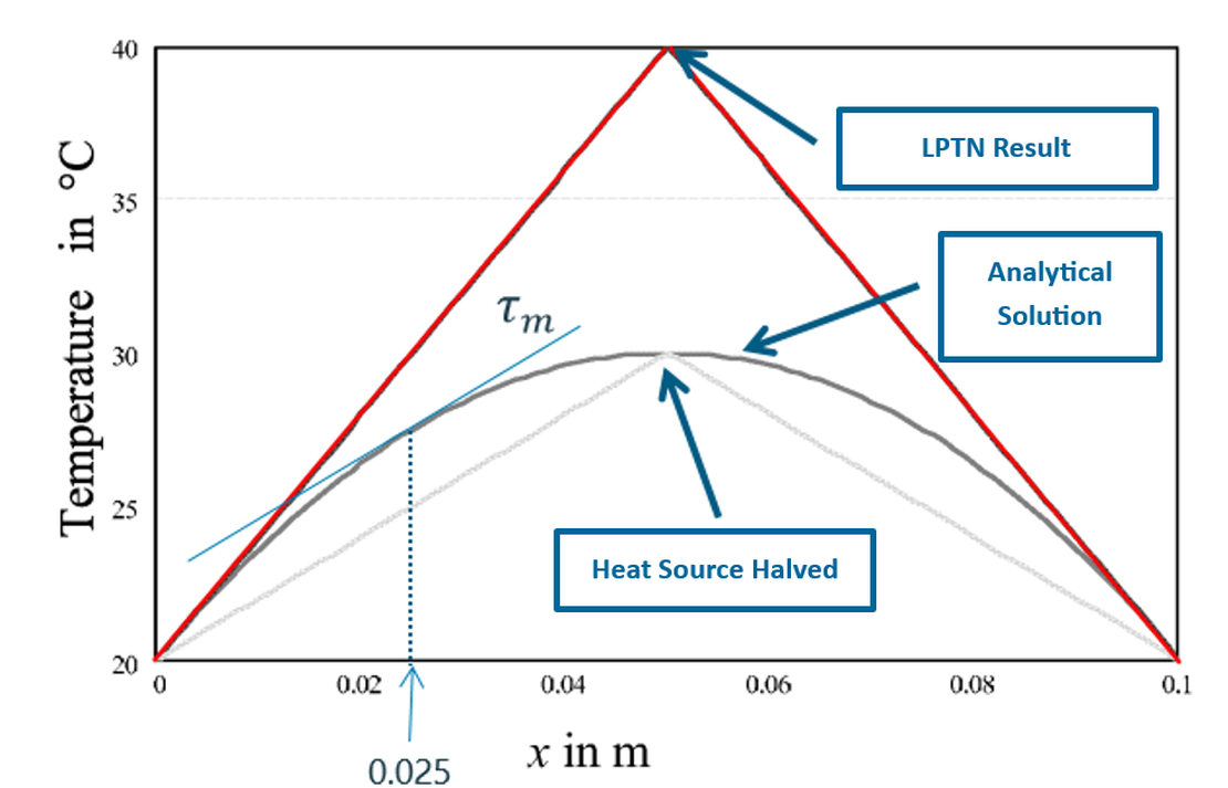
Figure 4: Comparison of Temperature Results Between the Heat Source Halving Method and Analytical Solution Using the LPTN Method

If both boundary temperatures are equal, the midpoint will correspond to the location of maximum temperature.
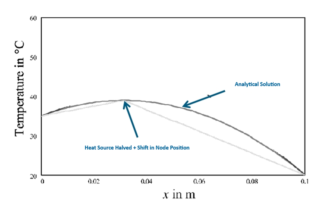
However, when the boundary temperatures differ, the maximum temperature point shifts toward the hotter boundary. Its location can be derived from the analytical solution:

x_{\text{max}} = \frac{L(T_1 - T_2)}{\dot{q}L^2 / (2k) + (T_1 - T_2)} \tag{5}

To determine the correct maximum temperature, the nodal position within the thermal network can be iteratively adjusted based on the boundary temperatures until convergence is achieved.

Figure 5: Comparison of Temperature Results Between the Heat Source Halving Method + Node Position Shift and the Analytical Solution

2.2 Additional Thermal Resistance

The governing equation for heat conduction with internal heat generation is the Poisson equation. Owing to its linearity, it can be decomposed into two independent problems using the principle of superposition:

A problem representing pure conduction (no heat source).
A problem representing the temperature increment due to the heat source.

The subproblem without heat sources aligns well with the LPTN assumption. The second subproblem, representing heat generation, can be modeled as an additional corrective thermal resistance in the network.

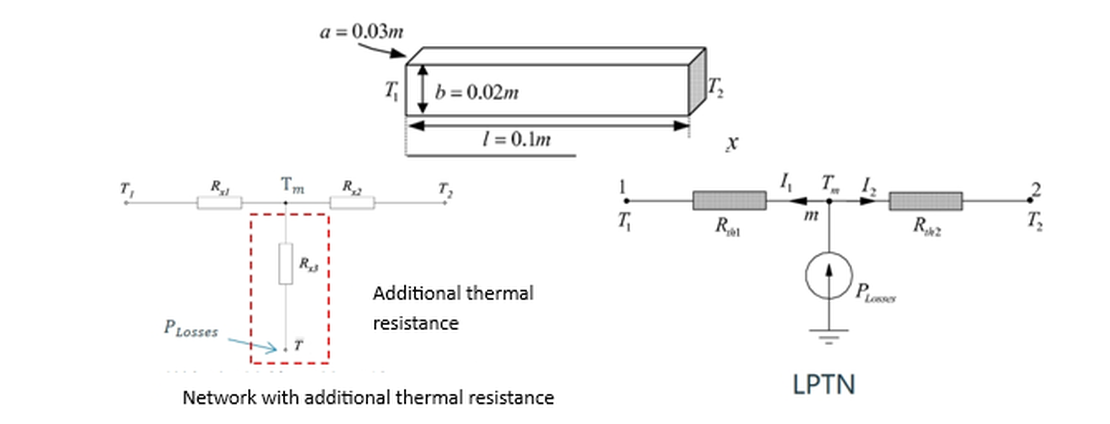
Figure 6: Temperature-Corrected Thermal Network Diagram

For this modified network, the additional correction resistance $R_{x3}$ can be derived as follows:

\frac{d^2 T}{dx^2} = -\frac{\dot{q}}{k} \tag{6}

With boundary conditions:

T(0) = 0, \quad T(L) = 0 \tag{7}

Integrating yields the average correction temperature $\bar{T}$ :

\bar{T} = \frac{\dot{q}L^2}{12k} \tag{8}

The equivalent correction resistance can be obtained from energy balance considerations:

R_{x3} = -\frac{L}{6kA} \tag{9}

The negative value of $R_{x3}$ implies an apparent heat flow from a lower to a higher temperature region, physically unrealistic but computationally effective. It offsets the LPTN’s temperature overestimation by lowering the predicted midpoint temperature.

If $\dot{q} = 0$ , the equation reduces to the traditional LPTN model without internal sources.

2.3 Increasing Network Nodes

Because traditional LPTN models lump the entire geometry into a few nodes, they lose spatial resolution and are less accurate for systems with distributed heat generation. Increasing the number of nodes helps capture this spatial dependence more effectively.

In the limiting case of an infinite number of nodes, the analytical temperature distribution can be reproduced exactly. However, this approach increases computational cost and modeling complexity.

Modern tools such as shonTA employ flexible templates that allow arbitrary node discretization along both axial and radial directions. With parallel processing support, these models can balance accuracy and efficiency.

shonTA motor template showing a) rotor’s circumferential projection; b) discrete node diagram; c) temperature field contour plot — Figure 7: shonTA motor template showing a) the rotor’s circumferential geometric projection; b) the rotor’s discrete node diagram; c) the rotor’s temperature field contour plot

3. 总结

When volumetric heat sources are present, conventional thermal network methods tend to overpredict temperatures compared to analytical results.
Three practical correction strategies are available:

Heat Source Correction Method
- Adjusts total heat generation (e.g., halving the heat source).
- Matches maximum temperature but reduces total system energy.
- Requires node relocation if boundary temperatures differ.
Additional Thermal Resistance Method
- Introduces a corrective negative resistance to balance overestimation.
- Ensures a more accurate average temperature.
Increasing Network Nodes
- Improves spatial accuracy.
- Increases computational cost and modeling effort.

These techniques collectively enhance the reliability of the LPTN method for systems with internal heat generation, such as electrical machines and high-density thermal systems.

References

[1] Dieter Gerling, Gurakuq Dajaku. Novel lumped-parameter thermal model for electrical systems. 2005.
[2] R. Wrobel, P. H. Mellor. A General Cuboidal Element for Three-Dimensional Thermal Modelling. IEEE Transactions on Magnetics, 2010.

联系我们

申请免费试用或向我们咨询任何产品相关问题

Improving Accuracy in the Lumped-Parameter Thermal Network (LPTN) Method (2/2)